Distributed Lag Linear and Non-Linear Models in R: The Package dlnm
Distributed lag/non-linear models (DLNMs) is a modelling framework to describe simultaneously a non-linear and a delayed effects between predictors and an outcome, a dependency defined as exposure-lag-response (outcome) association in time series data. This methodology rests on the definition of a crossbasis, a bi-dimensional functional space expressed by the combination of two sets of basis functions, which specify the relationships in the dimensions of predictor and lags, respectively (Gasparrini 2011).
What is DLNM?
In case of protracted exposures, the data can be structured by the partition in equally-spaced time periods, defining a series of exposure events and outcomes realizations. This methodology allows the effect of a single exposure event to be distributed over a specific period of time, using several parameters to explain the contributions at different lags, thus providing a comprehensive picture of the time-course of the exposure-response relationship.
“Non-linear” Relationship: The link between exposure and outcome might not be a straight line. Maybe very high temperatures drastically increase health risks, while mild temperatures don’t have much effect. DLNMs use flexible curves (like splines) to model these more complex, curvy relationships.
Lagged Effects: Instead of assuming an exposure affects health only on the same day, DLNMs captures delayed effects—like a heat wave that might cause more hospital admissions not just today, but also in the following days or weeks.
Traditionally, an epidemiological approach is to study the exposure-response relationship. The DLNM framework extend it by adding the lag-response relationship to construct the so-called dependency exposure-lag-response relationship, characterized by the bi-dimensional space of predictor and lag.
Specifically, two set of basis functions are chosen independently for modelling the exposure and lag-response relationships. These are then combined through a special tensor product defined by bi-dimensional cross-basis functions. The choice of the two sets of functions determines the shape of the relationship in each dimension. DLMs can be considered special cases of the more general DLNMs, when the exposure-response is assumed linear.
In the standard definition of the DLM/DLNM modelling framework, models are fitted with common regression methods, such as generalized linear models (GLMs) or Cox proportional hazard models. The functions in the dlnm package can be used more generally to facilitate the computation and interpretation of associations estimated from regression models, beyod the specific case of distributed lag modelling. Specifically, the functions can be applied to obtain predictions and plots of point estimates and measures of uncertainty for linear or non-linear unlagged relationships, estimated from either unpenalized (e.g., GLMs and Cox models) or penalized (GAMs) models.
The first step for performing DLMs or DLNMs consists of the choice of two sets of basis functions for modelling the exposure-lag-response association. Any kind of function determining completely known parametric transformations of the predictor can be used, and several options are available in the dlnm package. All the functions are meant to be called internally by onebasis() and crossbasis() and not directly run by the users.
Since version 2.0.0 of dlnm, onebasis() simply acts as a wrapper to other functions. The function has a first argument x for the predictor variable (i.e. ambient temperature), and another argument fun for specifying the basis function to be called internally, whose arguments are passed through the ellipsis argument ‘…’.
The function crossbasis() is the main function in the package dlnm. It calls onebasis() internally to generate the basis matrices for exposure-response and lag-response relationships, and combines them through a special tensor product in order to create the cross-basis, which specifies the exposure-lag-response dependency simultaneously in the two dimensions. The class of the first argument x of crossbasis() defines how the data are interpreted. If a vector, x is assumed to represent an equally-spaced, complete and ordered series of observations in a time series framework. If a matrix, x is assumed to represent a series of exposure histories for each observation (rows) and lag (columns). The lag period can be defined through the second argument lag. The two arguments argvar and arglag contain lists of arguments, each of them to be passed to onebasis() to build the matrices for the exposure-response and lag-response relationships respectively. The additional argument group, used only for time series data, defines groups of observations to be considered as individual unrelated series, and may be useful for example in seasonal analyses.
The function crosspred(): The interpretation of estimated parameters is usually complex for non-trivial basis transformations in DLMs, and virtually impossible in bi-dimensional DLNMs. The function crosspred() facilitates the interpretation by predicting the association for a grid of predictor and lag values, chosen by default or directly by the user. The function creates the same basis or cross-basis functions for the chosen predictor and lag values, extracts the related parameters estimated in the regression model, and generates predictions with associated standard errors and confidence intervals.
Practical example
We will use the chicagoNMMAPS as an example of analysis. The example refers to the effects on all-cause mortality of two environmental factors, air pollution (ozone) and temperature, in the city of Chicago during the period 1987-2000.
pacman::p_load(
  rio,
  here,
  DT,
  dlnm,
  splines,
  survival,
  sjPlot,
  tidyverse
)data(chicagoNMMAPS)
datatable(chicagoNMMAPS)A model for time series data may be generally represented by:
\[ g(\mu_i) = \alpha + \sum_{j=1}^J s_j\bigl(x_{ij}, \beta_j\bigr) + \sum_{k=1}^K \gamma_k\,u_{ik} \]
In the illustrative example on Chicago data, the outcome Yt is daily death counts, assumed to originate from a so-called overdispersed Poisson distribution with E(Y) = μ, V(Y) = \(\phi\) μ, and a canonical log-link. The non-linear and delayed effects of ozone and temperature are modeled through as particular functions sj which define the relationship along the two dimensions of predictor and lags. Generally, non-linear exposure-response dependencies are expressed in regression models through appropriate functions s. The main choices typically rely on functions describing smooth curves, like polynomials or spline functions. All of these functions apply a transformation of the original predictor to generate a set of transformed variables included in the model as linear terms.

The DLNMs framework introduced in this paper is developed for time series data. The general expression of the basic model in allows this methodology to be applied to any family distribution and link function within (generalized) linear models (GLM), with extensions to generalized additive models (GAM) or models based on generalized estimating equations (GEE) (Perperoglou et al. 2019). However, the current implementation of DLNMs requires single series of equally-spaced, complete and ordered data.
Specifying a DLNM
basis.o3 <- crossbasis(
  chicagoNMMAPS$o3,
  lag = 10,
  argvar = list(fun = "thr", thr.value = 40.3, side = "h"),
  arglag = list(fun = "strata", breaks = c(2, 6))
)

klag <- exp(((1 + log(30)) / 4 * 1:3) - 1)
basis.temp <- crossbasis(
  chicagoNMMAPS$temp,
  lag = 30,
  argvar = list(fun = "bs", degree = 3, df = 6),
  arglag = list(knots = klag)
)

summary(basis.o3)
CROSSBASIS FUNCTIONS
observations: 5114
range: -0.8319944 to 65.80827
lag period: 0 10
total df: 3
BASIS FOR VAR:
fun: thr
thr.value: 40.3
side: h
intercept: FALSE
BASIS FOR LAG:
fun: strata
df: 3
breaks: 2 6
ref: 1
intercept: TRUE summary(basis.temp)CROSSBASIS FUNCTIONS
observations: 5114
range: -26.66667 to 33.33333
lag period: 0 30
total df: 30
BASIS FOR VAR:
fun: bs
knots: 1.666667 10.55556 19.44444
degree: 3
intercept: FALSE
Boundary.knots: -26.66667 33.33333
BASIS FOR LAG:
fun: ns
knots: 1.105502 3.322105 9.983144
intercept: TRUE
Boundary.knots: 0 30 - The first argument x of crossbasis() is the predictor series, in this case chicagoNMMAPS\(o3 and chicagoNMMAPS\)temp. The values in x are expected to represent an equally-spaced and ordered series, with the interval defining the lag unit
- The cross-basis for ozone comprises a threshold function for the space of the predictor, with a linear relationship beyond 40.3 μgr/m3, and a dummy parameterization assuming constant distributed lag effects along the strata of lags 0-1, 2-5 and 6-10 ().
- In contrast, the options for temperature are a cubic spline with 6 df (knots at equally-spaced percentiles by default) centered at 25°C, and a natural cubic spline (lagtype = “ns” by default) with 5 df (knots at equally-spaced values in the log scale of lags by default), up to a maximum of 30 lags.
The cross-basis matrices can be included in the model formula of a common regression function in order to estimate the corresponding parameters η in (5). In the example, the final model includes also a natural cubic spline with 7 df/year to model the seasonal and long time trend components and a factor for day of the week, specified by the function ns() in the package splines, which needs to be loaded in the session. The code is:
model <- glm(
  death ~ basis.temp + basis.o3 + ns(time, 7 * 14) + dow,
  family = quasipoisson(),
  chicagoNMMAPS
)| death | |||
| Predictors | Incidence Rate Ratios | CI | p |
| (Intercept) | 129.22 | 82.15 – 203.14 | <0.001 |
| basis tempv1 l1 | 0.91 | 0.81 – 1.01 | 0.070 |
| basis tempv1 l2 | 1.03 | 0.97 – 1.09 | 0.409 |
| basis tempv1 l3 | 0.98 | 0.91 – 1.06 | 0.659 |
| basis tempv1 l4 | 1.02 | 0.91 – 1.14 | 0.781 |
| basis tempv1 l5 | 0.99 | 0.92 – 1.06 | 0.734 |
| basis tempv2 l1 | 0.95 | 0.88 – 1.02 | 0.138 |
| basis tempv2 l2 | 0.99 | 0.96 – 1.03 | 0.737 |
| basis tempv2 l3 | 0.99 | 0.95 – 1.04 | 0.719 |
| basis tempv2 l4 | 1.04 | 0.96 – 1.12 | 0.325 |
| basis tempv2 l5 | 0.97 | 0.93 – 1.02 | 0.259 |
| basis tempv3 l1 | 0.88 | 0.82 – 0.96 | 0.003 |
| basis tempv3 l2 | 1.00 | 0.96 – 1.05 | 0.865 |
| basis tempv3 l3 | 0.98 | 0.93 – 1.04 | 0.491 |
| basis tempv3 l4 | 1.02 | 0.94 – 1.12 | 0.622 |
| basis tempv3 l5 | 0.98 | 0.93 – 1.03 | 0.393 |
| basis tempv4 l1 | 0.91 | 0.84 – 0.98 | 0.015 |
| basis tempv4 l2 | 1.00 | 0.96 – 1.04 | 0.964 |
| basis tempv4 l3 | 0.96 | 0.91 – 1.01 | 0.162 |
| basis tempv4 l4 | 1.10 | 1.01 – 1.19 | 0.029 |
| basis tempv4 l5 | 0.94 | 0.90 – 0.99 | 0.023 |
| basis tempv5 l1 | 0.76 | 0.70 – 0.82 | <0.001 |
| basis tempv5 l2 | 0.99 | 0.95 – 1.04 | 0.823 |
| basis tempv5 l3 | 0.95 | 0.89 – 1.01 | 0.081 |
| basis tempv5 l4 | 1.07 | 0.98 – 1.17 | 0.155 |
| basis tempv5 l5 | 0.96 | 0.90 – 1.01 | 0.136 |
| basis tempv6 l1 | 1.21 | 1.10 – 1.32 | <0.001 |
| basis tempv6 l2 | 0.98 | 0.93 – 1.03 | 0.470 |
| basis tempv6 l3 | 0.89 | 0.83 – 0.95 | <0.001 |
| basis tempv6 l4 | 1.33 | 1.20 – 1.47 | <0.001 |
| basis tempv6 l5 | 0.86 | 0.80 – 0.91 | <0.001 |
| basis o3v1 l1 | 1.00 | 1.00 – 1.00 | <0.001 |
| basis o3v1 l2 | 1.00 | 1.00 – 1.00 | 0.007 |
| basis o3v1 l3 | 1.00 | 1.00 – 1.00 | <0.001 |
| time [1st degree] | 1.09 | 0.89 – 1.33 | 0.395 |
| time [2nd degree] | 1.17 | 0.90 – 1.53 | 0.237 |
| time [3rd degree] | 1.09 | 0.86 – 1.39 | 0.467 |
| time [4th degree] | 1.16 | 0.90 – 1.50 | 0.247 |
| time [5th degree] | 1.15 | 0.91 – 1.46 | 0.236 |
| time [6th degree] | 1.13 | 0.89 – 1.44 | 0.304 |
| time [7th degree] | 1.07 | 0.85 – 1.35 | 0.557 |
| time [8th degree] | 1.25 | 0.99 – 1.59 | 0.065 |
| time [9th degree] | 1.05 | 0.82 – 1.35 | 0.686 |
| time [10th degree] | 1.06 | 0.82 – 1.37 | 0.662 |
| time [11th degree] | 1.13 | 0.88 – 1.45 | 0.350 |
| time [12th degree] | 1.17 | 0.92 – 1.48 | 0.205 |
| time [13th degree] | 1.06 | 0.84 – 1.35 | 0.601 |
| time [14th degree] | 1.12 | 0.89 – 1.42 | 0.337 |
| time [15th degree] | 1.08 | 0.86 – 1.37 | 0.504 |
| time [16th degree] | 1.15 | 0.90 – 1.47 | 0.267 |
| time [17th degree] | 1.07 | 0.83 – 1.37 | 0.619 |
| time [18th degree] | 1.21 | 0.94 – 1.54 | 0.136 |
| time [19th degree] | 1.04 | 0.82 – 1.32 | 0.774 |
| time [20th degree] | 1.38 | 1.09 – 1.74 | 0.007 |
| time [21st degree] | 1.04 | 0.82 – 1.32 | 0.729 |
| time [22nd degree] | 1.12 | 0.89 – 1.42 | 0.338 |
| time [23rd degree] | 1.12 | 0.88 – 1.43 | 0.372 |
| time [24th degree] | 1.04 | 0.81 – 1.34 | 0.748 |
| time [25th degree] | 1.18 | 0.92 – 1.51 | 0.190 |
| time [26th degree] | 1.11 | 0.88 – 1.42 | 0.375 |
| time [27th degree] | 1.08 | 0.86 – 1.37 | 0.507 |
| time [28th degree] | 1.17 | 0.93 – 1.48 | 0.189 |
| time [29th degree] | 1.08 | 0.85 – 1.37 | 0.548 |
| time [30th degree] | 1.18 | 0.92 – 1.51 | 0.191 |
| time [31st degree] | 1.04 | 0.81 – 1.33 | 0.769 |
| time [32nd degree] | 1.16 | 0.91 – 1.49 | 0.241 |
| time [33rd degree] | 1.08 | 0.85 – 1.37 | 0.533 |
| time [34th degree] | 1.28 | 1.01 – 1.62 | 0.038 |
| time [35th degree] | 1.00 | 0.79 – 1.27 | 0.994 |
| time [36th degree] | 1.13 | 0.89 – 1.43 | 0.329 |
| time [37th degree] | 1.08 | 0.85 – 1.37 | 0.552 |
| time [38th degree] | 1.03 | 0.80 – 1.32 | 0.821 |
| time [39th degree] | 1.10 | 0.86 – 1.40 | 0.465 |
| time [40th degree] | 1.17 | 0.92 – 1.49 | 0.193 |
| time [41st degree] | 1.02 | 0.81 – 1.30 | 0.844 |
| time [42nd degree] | 1.11 | 0.88 – 1.41 | 0.363 |
| time [43rd degree] | 1.31 | 1.04 – 1.66 | 0.024 |
| time [44th degree] | 1.03 | 0.81 – 1.31 | 0.825 |
| time [45th degree] | 1.21 | 0.94 – 1.56 | 0.131 |
| time [46th degree] | 1.13 | 0.89 – 1.45 | 0.324 |
| time [47th degree] | 1.12 | 0.88 – 1.42 | 0.365 |
| time [48th degree] | 1.21 | 0.96 – 1.53 | 0.116 |
| time [49th degree] | 1.04 | 0.82 – 1.32 | 0.738 |
| time [50th degree] | 1.14 | 0.90 – 1.45 | 0.284 |
| time [51st degree] | 1.14 | 0.90 – 1.45 | 0.291 |
| time [52nd degree] | 1.07 | 0.83 – 1.37 | 0.593 |
| time [53rd degree] | 1.17 | 0.91 – 1.49 | 0.223 |
| time [54th degree] | 1.10 | 0.87 – 1.40 | 0.442 |
| time [55th degree] | 1.26 | 1.00 – 1.60 | 0.053 |
| time [56th degree] | 1.18 | 0.93 – 1.49 | 0.174 |
| time [57th degree] | 1.08 | 0.85 – 1.37 | 0.541 |
| time [58th degree] | 1.12 | 0.88 – 1.43 | 0.366 |
| time [59th degree] | 1.26 | 0.98 – 1.63 | 0.078 |
| time [60th degree] | 1.02 | 0.79 – 1.30 | 0.899 |
| time [61st degree] | 1.11 | 0.87 – 1.40 | 0.412 |
| time [62nd degree] | 1.17 | 0.92 – 1.48 | 0.193 |
| time [63rd degree] | 0.96 | 0.76 – 1.21 | 0.716 |
| time [64th degree] | 1.13 | 0.89 – 1.43 | 0.314 |
| time [65th degree] | 1.06 | 0.83 – 1.35 | 0.643 |
| time [66th degree] | 1.07 | 0.84 – 1.38 | 0.588 |
| time [67th degree] | 1.02 | 0.79 – 1.30 | 0.904 |
| time [68th degree] | 1.19 | 0.94 – 1.51 | 0.146 |
| time [69th degree] | 1.21 | 0.96 – 1.53 | 0.117 |
| time [70th degree] | 0.93 | 0.73 – 1.17 | 0.531 |
| time [71st degree] | 1.16 | 0.91 – 1.47 | 0.221 |
| time [72nd degree] | 1.02 | 0.80 – 1.30 | 0.874 |
| time [73rd degree] | 1.03 | 0.80 – 1.32 | 0.832 |
| time [74th degree] | 1.01 | 0.79 – 1.30 | 0.919 |
| time [75th degree] | 1.12 | 0.88 – 1.43 | 0.343 |
| time [76th degree] | 1.05 | 0.83 – 1.33 | 0.699 |
| time [77th degree] | 1.21 | 0.95 – 1.53 | 0.119 |
| time [78th degree] | 0.97 | 0.77 – 1.23 | 0.801 |
| time [79th degree] | 1.03 | 0.80 – 1.32 | 0.825 |
| time [80th degree] | 1.10 | 0.86 – 1.42 | 0.440 |
| time [81st degree] | 1.06 | 0.82 – 1.36 | 0.666 |
| time [82nd degree] | 1.04 | 0.82 – 1.33 | 0.726 |
| time [83rd degree] | 1.13 | 0.90 – 1.43 | 0.291 |
| time [84th degree] | 1.31 | 1.03 – 1.66 | 0.026 |
| time [85th degree] | 1.06 | 0.84 – 1.35 | 0.620 |
| time [86th degree] | 1.01 | 0.79 – 1.29 | 0.961 |
| time [87th degree] | 1.05 | 0.82 – 1.36 | 0.685 |
| time [88th degree] | 1.00 | 0.79 – 1.28 | 0.981 |
| time [89th degree] | 1.05 | 0.83 – 1.34 | 0.692 |
| time [90th degree] | 1.35 | 1.06 – 1.70 | 0.013 |
| time [91st degree] | 0.88 | 0.70 – 1.11 | 0.283 |
| time [92nd degree] | 1.14 | 0.90 – 1.46 | 0.272 |
| time [93rd degree] | 1.01 | 0.79 – 1.29 | 0.937 |
| time [94th degree] | 1.03 | 0.81 – 1.33 | 0.788 |
| time [95th degree] | 1.06 | 0.83 – 1.35 | 0.651 |
| time [96th degree] | 1.08 | 0.92 – 1.27 | 0.357 |
| time [97th degree] | 1.20 | 0.73 – 1.95 | 0.473 |
| time [98th degree] | 1.00 | 0.92 – 1.09 | 0.994 |
| dow [Monday] | 1.04 | 1.03 – 1.05 | <0.001 |
| dow [Tuesday] | 1.03 | 1.02 – 1.04 | <0.001 |
| dow [Wednesday] | 1.01 | 1.00 – 1.02 | 0.010 |
| dow [Thursday] | 1.02 | 1.01 – 1.03 | 0.002 |
| dow [Friday] | 1.02 | 1.01 – 1.03 | <0.001 |
| dow [Saturday] | 1.02 | 1.01 – 1.03 | <0.001 |
| Observations | 5084 | ||
| R2 Nagelkerke | 0.657 | ||
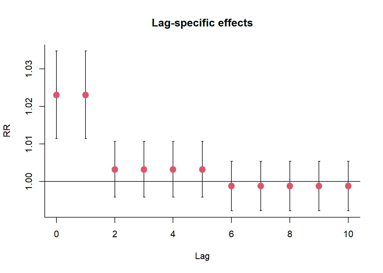
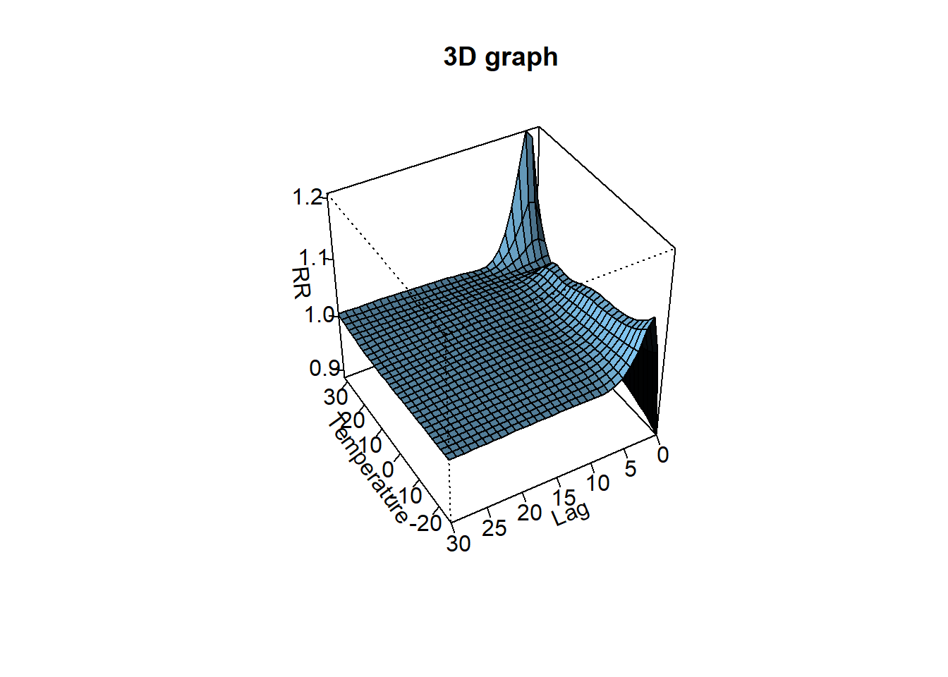
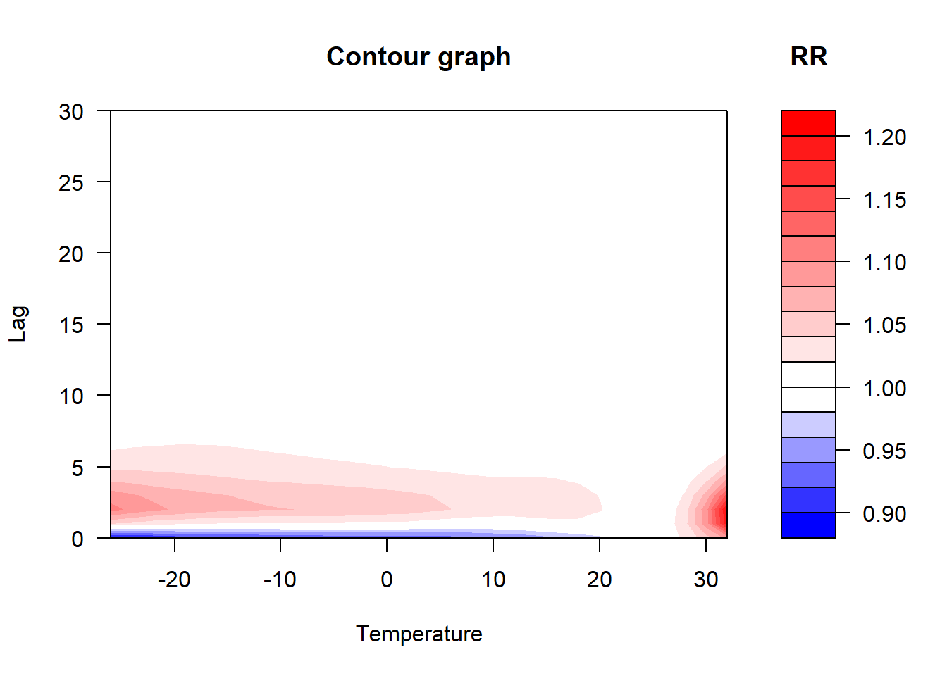
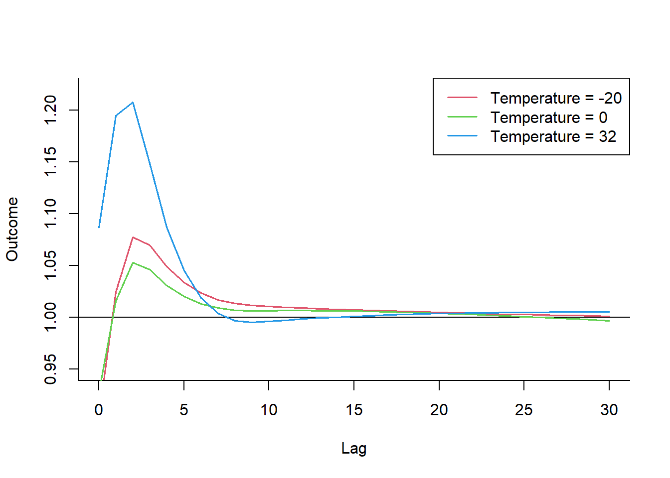
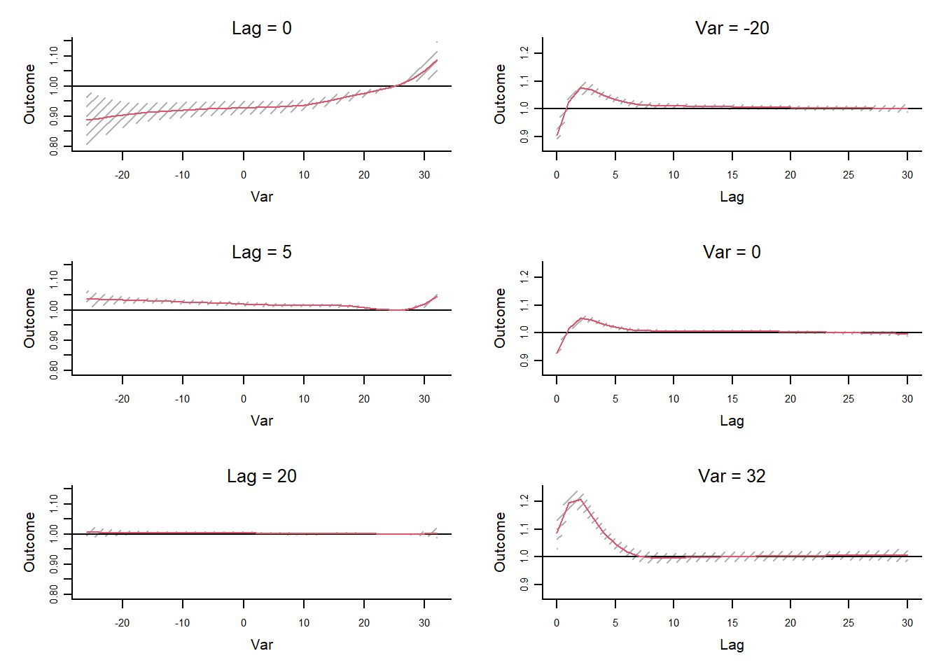
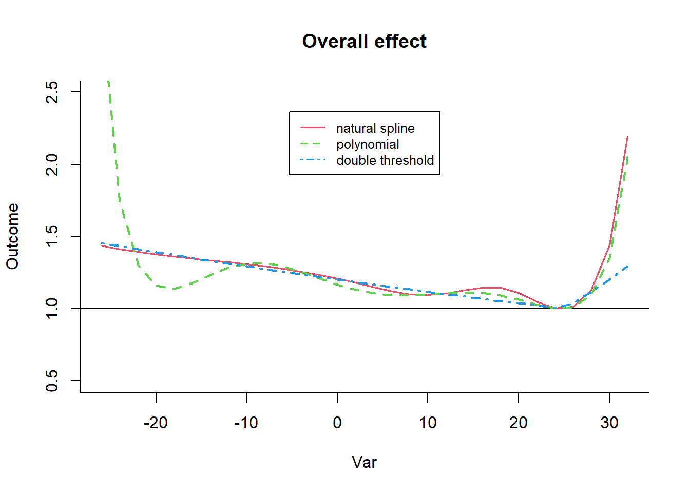
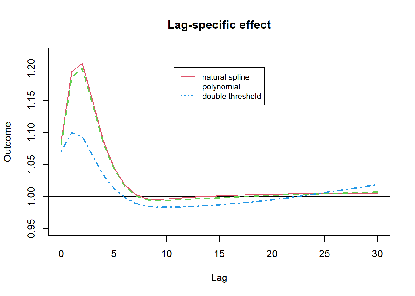
The bi-dimensional exposure-response relationship estimated by a DLNM may be difficult to summarize. The meaning of such parameters, which define the relationship along two dimensions, is not straightforward. Interpretation can be aided by the prediction of lag-specific effects on a grid of suitable exposure values and the L + 1 lags. In addition, the overall effects, predicted from exposure sustained over lags L to 0, can be computed by summing the lag-specific contributions.
Predicting from a DLNM
Predicted effects are computed in dlnm by the function crosspred(). The following code computes the prediction for ozone and temperature in the example:
pred.o3 <- crosspred(
basis.o3,
model,
at = c(0:65, 40.3, 50.3)
) # chose the integers from 0 to 65 μgr/m3 in ozone, plus the value of the chosen threshold and 10 units above (40.3 and 50.3 μgr/m3, respectively)
pred.temp <- crosspred(
basis.temp,
model,
by = 2, # rounded values within the temperature range with an increment of 2°C.
cen = 25
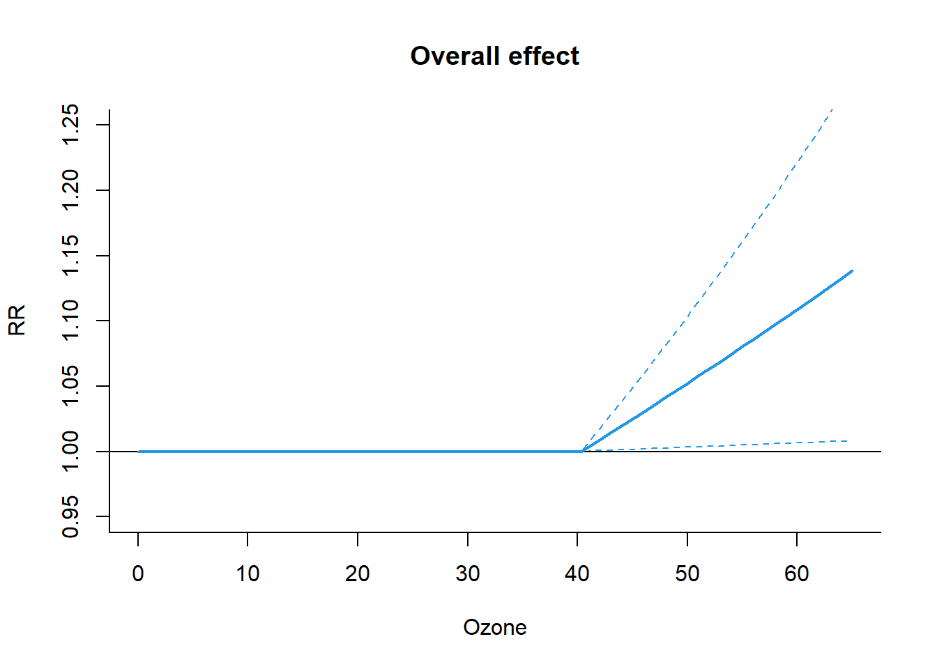
)The results stored in the crosspred object can be directly accessed to obtain specific figures or customized graphs other than those produced by dlnm plotting functions. For example, the overall effect for the 10-unit increase in ozone, expressed as RR and 95% confidence intervals, can be derived by:
pred.o3$allRRfit["50.3"] # RR = 1.05387 50.3
1.05387 cbind(pred.o3$allRRlow, pred.o3$allRRhigh)["50.3", ] # combine low and high value[1] 1.003354 1.106930source(here("2-dlnm/dlnm_example.R"))CROSSBASIS FUNCTIONS
observations: 5114
range: -26.66667 to 33.33333
lag period: 0 30
total df: 30
BASIS FOR VAR:
fun: bs
knots: 1.666667 10.55556 19.44444
degree: 3
intercept: FALSE
Boundary.knots: -26.66667 33.33333
BASIS FOR LAG:
fun: ns
knots: 1.105502 3.322105 9.983144
intercept: TRUE
Boundary.knots: 0 30