Rows: 18
Columns: 8
$ Author               <chr> "Call et al.", "Cavanagh et al.", "DanitzOrsillo"…
$ TE                   <dbl> 0.7091362, 0.3548641, 1.7911700, 0.1824552, 0.421…
$ seTE                 <dbl> 0.2608202, 0.1963624, 0.3455692, 0.1177874, 0.144…
$ RiskOfBias           <chr> "high", "low", "high", "low", "low", "low", "high…
$ TypeControlGroup     <chr> "WLC", "WLC", "WLC", "no intervention", "informat…
$ InterventionDuration <chr> "short", "short", "short", "short", "short", "sho…
$ InterventionType     <chr> "mindfulness", "mindfulness", "ACT", "mindfulness…
$ ModeOfDelivery <chr> "group", "online", "group", "group", "online", "g…Meta-regression introduction
Overview about meta-analysis
Meta-analysis is a technique to combine the results of multiple studies to arrive at a single conclusion about the overall effect of an intervention or exposure. This is particularly useful when individual studies may have small sample sizes or conflicting results (Harrer et al. 2021).
-
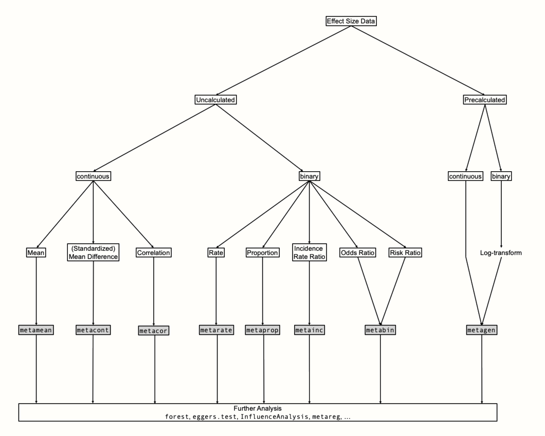
To perform a meta-analysis, we have to find an
effect sizewhich can be summarized across all studies. Sometimes, such effect sizes can be directly extracted from the publication; more often, we have to calculate them from other data reported in the studies.- Observational studies:
- Mean:
n,mean,sd - Proportion:
n,event - Correlation coefficients:
n,cor
- Mean:
- Experimental studies:
- Mean differences:
n.e,mean.e,sd.e,n.c,mean.c,sd.c - Risk and Odds Ratios:
n.e,event.e,n.c,event.c - Incidence Rate Ratios:
event.e,time.e,event.c,time.c - Hazard Ratio: extract the log-hazard ratio and its corresponding standard error from all studies, then performing a meta-analysis using inverse-variance pooling
- Mean differences:
- Observational studies:
- The Fixed-Effect and Random-Effects Model
- The fixed-effect model assumes that all effect sizes stem from a single, homogeneous population. It states that all studies share the same true effect size. The fixed-effect model assumes that all our studies are part of a homogeneous population and that
the only causefor differences in observed effects is thesampling error of studies. - The random-effects model assumes that
there is not only one true effect sizebut a distribution of true effect sizes. The goal of the random-effects model is therefore not to estimate the one true effect size of all studies, but the mean of the distribution of true effects.
- The fixed-effect model assumes that all effect sizes stem from a single, homogeneous population. It states that all studies share the same true effect size. The fixed-effect model assumes that all our studies are part of a homogeneous population and that
Meta-regression
Meta-regression is a meta-analysis that uses regression analysis to combine, compare, and synthesize research findings from multiple studies while adjusting for the effects of available covariates on a response variable.
Normal linear regression models use the ordinary least squares (OLS) method to find the regression line that fits the data best. In meta-regression, a modified method called weighted least squares (WLS) is used, which makes sure that studies with a smaller standard error are given a higher weight.
m.gen <- metagen(
  TE = TE,
  seTE = seTE,
  studlab = Author,
  data = ThirdWave,
  sm = "SMD",
  fixed = FALSE,
  random = TRUE,
  method.tau = "REML",
  method.random.ci = "HK",
  title = "Third Wave Psychotherapies"
)
Warning: Use argument 'common' instead of 'fixed' (deprecated).Using meta-regression, we want to examine if the publication year of a study can be used to predict its effect size
#fmt: skip
year <- c(2014, 1998, 2010, 1999, 2005, 2014,
          2019, 2010, 1982, 2020, 1978, 2001,
          2018, 2002, 2009, 2011, 2011, 2013)
m.gen.reg <- metareg(m.gen, ~year)
m.gen.reg
Mixed-Effects Model (k = 18; tau^2 estimator: REML)

tau^2 (estimated amount of residual heterogeneity):     0.0188 (SE = 0.0226)
tau (square root of estimated tau^2 value):             0.1371
I^2 (residual heterogeneity / unaccounted variability): 29.26%
H^2 (unaccounted variability / sampling variability):   1.41
R^2 (amount of heterogeneity accounted for):            77.08%

Test for Residual Heterogeneity:
QE(df = 16) = 27.8273, p-val = 0.0332

Test of Moderators (coefficient 2):
F(df1 = 1, df2 = 16) = 9.3755, p-val = 0.0075

Model Results:

         estimate       se     tval  df    pval     ci.lb     ci.ub
intrcpt  -36.1546  11.9800  -3.0179  16  0.0082  -61.5510  -10.7582  **
year       0.0183   0.0060   3.0619  16  0.0075    0.0056    0.0310  **

---
Signif. codes:  0 '***' 0.001 '**' 0.01 '*' 0.05 '.' 0.1 ' ' 1
In the first line, the output tells us that a mixed-effects model has been fitted to the data, just as intended. The next few lines provide details on the amount of heterogeneity explained by the model. We see that the estimate of the residual heterogeneity variance, the variance that is not explained by the predictor, is \(\hat\tau^2_{\text{unexplained}}=\) 0.019.
The output also provides us with an \(I^2\) equivalent, which tells us that after inclusion of the predictor, 29.26% of the variability in our data can be attributed to the remaining between-study heterogeneity. In the normal random-effects meta-analysis model, we found that the \(I^2\) heterogeneity was 63%, which means that the predictor was able to “explain away” a substantial amount of the differences in true effect sizes.
In the last line, we see the value of \(R^2_*\), which in our example is 77%. This means that 77% of the difference in true effect sizes can be explained by the publication year, a value that is quite substantial.
The next section contains a Test for Residual Heterogeneity, which is essentially the \(Q\)-test. Now, we test if the heterogeneity not explained by the predictor is significant. We see that this is the case, with \(p\) = 0.03.
The next part shows the Test of Moderators. We see that this test is also significant (\(p\) = 0.0075). This means that our predictor, the publication year, does indeed influence the studies’ effect size.
The last section provides more details on the estimated regression coefficients. The first line shows the results for the intercept (intrcpt). This is the expected effect size (in our case: Hedges’ \(g\)) when our predictor publication year is zero. In our example, this represents a scenario which is, arguably, a little contrived: it shows the predicted effect of a study conducted in the year 0, which is \(\hat{g}=\) -36.15. This serves as yet another reminder that good statistical models do not have to be a perfect representation of reality; they just have to be useful.
The coefficient we are primarily interested in is the one in the second row. We see that the model’s estimate of the regression weight for year is 0.01. This means that for every additional year, the effect size \(g\) of a study is expected to rise by 0.01. Therefore, we can say that the effect sizes of studies have increased over time. The 95% confidence interval ranges from 0.005 to 0.3, showing that the effect is significant.
The {meta} package allows us to visualize a meta-regression using the bubble function. This creates a bubble plot, which shows the estimated regression slope, as well as the effect size of each study. To indicate the weight of a study, the bubbles have different sizes, with a greater size representing a higher weight.
To produce a bubble plot, we only have to plug our meta-regression object into the bubble function. Because we also want study labels to be displayed, we set studlab to TRUE.
bubble(m.gen.reg, studlab = TRUE)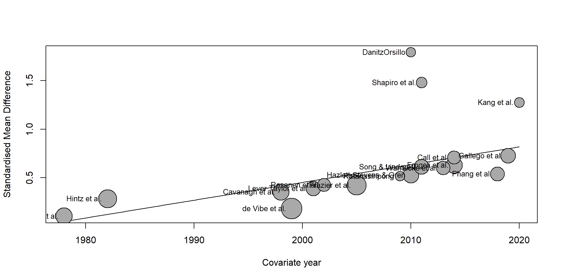
Multiple Meta-Regression in R
- The analysis is conducted using {metafor} package. This package provides a vast array of advanced functionality for meta-analysis, along with a great documentation
Note
The “MVRegressionData” Data Set
The MVRegressionData data set is included directly in the {dmetar} package. If you have installed {dmetar}, and loaded it from your library, running data(MVRegressionData) automatically saves the data set in your R environment. The data set is then ready to be used. If you do not have {dmetar} installed, you can download the data set as an .rda file from the Internet, save it in your working directory, and then click on it in your R Studio window to import it.
Rows: 36
Columns: 6
$ yi         <dbl> 0.09437543, 0.09981923, 0.16931607, 0.17511107, 0.27301641,…
$ sei        <dbl> 0.1959031, 0.1918510, 0.1193179, 0.1161592, 0.1646946, 0.17…
$ reputation <dbl> -11, 0, -11, 4, -10, -9, -8, -8, -8, 0, -5, -5, -4, -4, -3,…
$ quality    <dbl> 6, 9, 5, 9, 2, 10, 6, 3, 10, 3, 1, 5, 10, 2, 1, 2, 4, 1, 8,…
$ pubyear    <dbl> -0.85475360, -0.75277184, -0.66048349, -0.56304843, -0.4308…
$ continent  <fct> 1, 0, 1, 0, 1, 0, 0, 0, 0, 0, 0, 1, 0, 0, 0, 0, 0, 0, 0, 1,…
Checking for Multi-Collinearity
           reputation    quality    pubyear
reputation  1.0000000  0.3015694  0.3346594
quality     0.3015694  1.0000000 -0.1551123
pubyear     0.3346594 -0.1551123  1.0000000
# Visualizae the result
MVRegressionData[, c("reputation", "quality", "pubyear")] %>%
chart.Correlation()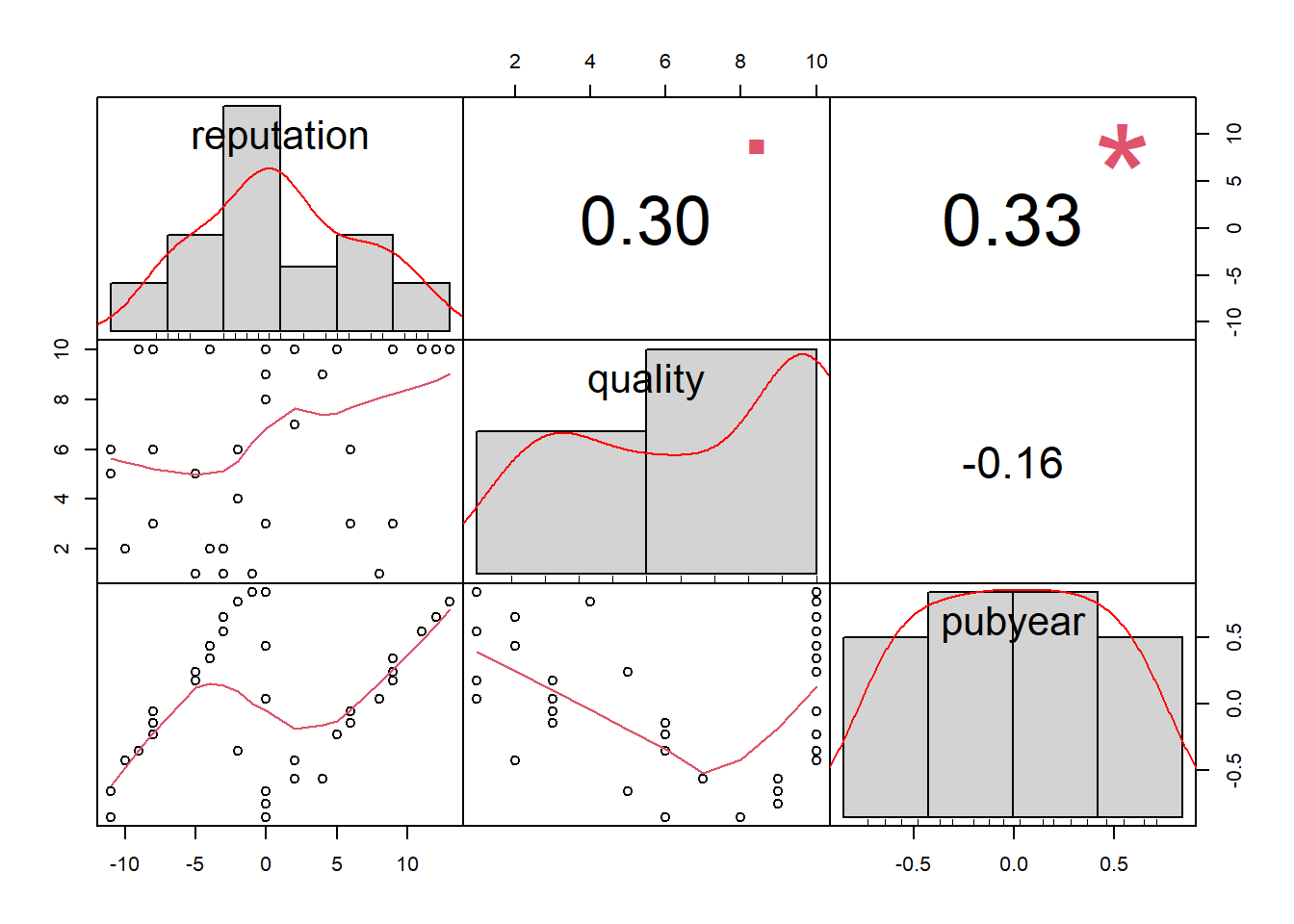
Fitting a Multiple Meta-Regression Model
Using only quality as a predictor
m.qual <- rma(
  yi = yi,
  sei = sei,
  data = MVRegressionData,
  method = "ML",
  mods = ~quality,
  test = "knha"
)

m.qual
Mixed-Effects Model (k = 36; tau^2 estimator: ML)

tau^2 (estimated amount of residual heterogeneity):     0.0667 (SE = 0.0275)
tau (square root of estimated tau^2 value):             0.2583
I^2 (residual heterogeneity / unaccounted variability): 60.04%
H^2 (unaccounted variability / sampling variability):   2.50
R^2 (amount of heterogeneity accounted for):            7.37%

Test for Residual Heterogeneity:
QE(df = 34) = 88.6130, p-val < .0001

Test of Moderators (coefficient 2):
F(df1 = 1, df2 = 34) = 3.5330, p-val = 0.0688

Model Results:

         estimate      se    tval  df    pval    ci.lb   ci.ub
intrcpt    0.3429  0.1354  2.5318  34  0.0161   0.0677  0.6181  *
quality    0.0356  0.0189  1.8796  34  0.0688  -0.0029  0.0740  .

---
Signif. codes:  0 '***' 0.001 '**' 0.01 '*' 0.05 '.' 0.1 ' ' 1
Next, we include reputation as a predictor
m.qual.rep <- rma(
  yi = yi,
  sei = sei,
  data = MVRegressionData,
  method = "ML",
  mods = ~ quality + reputation,
  test = "knha"
)

m.qual.rep
Mixed-Effects Model (k = 36; tau^2 estimator: ML)

tau^2 (estimated amount of residual heterogeneity):     0.0238 (SE = 0.0161)
tau (square root of estimated tau^2 value):             0.1543
I^2 (residual heterogeneity / unaccounted variability): 34.62%
H^2 (unaccounted variability / sampling variability):   1.53
R^2 (amount of heterogeneity accounted for):            66.95%

Test for Residual Heterogeneity:
QE(df = 33) = 58.3042, p-val = 0.0042

Test of Moderators (coefficients 2:3):
F(df1 = 2, df2 = 33) = 12.2476, p-val = 0.0001

Model Results:

            estimate      se    tval  df    pval    ci.lb   ci.ub
intrcpt       0.5005  0.1090  4.5927  33  <.0001   0.2788  0.7222  ***
quality       0.0110  0.0151  0.7312  33  0.4698  -0.0197  0.0417
reputation    0.0343  0.0075  4.5435  33  <.0001   0.0189  0.0496  ***

---
Signif. codes: 0 '***' 0.001 '**' 0.01 '*' 0.05 '.' 0.1 ' ' 1anova(m.qual, m.qual.rep)
        df     AIC     BIC    AICc   logLik     LRT   pval      QE  tau^2
Full     4 19.4816 25.8157 20.7720  -5.7408                58.3042 0.0238
Reduced  3 36.9808 41.7314 37.7308 -15.4904 19.4992 <.0001 88.6130 0.0667
             R^2
Full
Reduced 64.3197%
The anova function performs a likelihood ratio test, the results of which we can see in the LRT column. The test is highly significant, which means that that the new full model indeed provides a better fit.
https://www.youtube.com/watch?v=xBJGUP8t4t8
References
Harrer, Mathias, Pim Cuijpers, Furukawa Toshi A, and David D Ebert. 2021. Doing Meta-Analysis with R: A Hands-on Guide. 1st ed. Boca Raton, FL; London: Chapman & Hall/CRC Press.