# https://github.com/gasparrini/2012_gasparrini_StatMed_Rcodedata
pacman::p_load(
  rio,
  here,
  dlnm,
  splines,
  survival,
  survminer,
  coxme,
  sjPlot,
  tidyverse
)Explore the association of temperature exposure with the mental health outcome
Load package and data
data <- import(here("data/Lea data_wide.dta"))The goal is to reshape the dataset from long into wide format, and then later use the DLNM. Currently, the dataset is already structured in a case-crossover design, with depression and anxiety as the two outcomes of interest and max_temp as the exposure variable. Each woman (unique_caseid) has 60 observations, divided across 4 control_lags, with one case period (control_lag==0) and three control periods, always one week apart from the interview_date. The daily_date represents the date. The goal is to only have one row per woman to allow analysis for the lags. dhscc is the country variable.
The same daily_dates can appear multiple times for a single woman but under different control_lags. This overlap occurs because, when setting up the case-crossover design, we agreed to use the interview date and take 1, 2, and 3 weeks prior as control periods, always including 14 days of temperature exposure. For example, in the case of unique_caseid “1 9 01_MZ”, the original interview_date was 31.07.2022. Based on this, I counted back one, two, and three weeks to determine the interview_dates for the control periods. Since the DHS mental health assessment refers to the past two weeks (“In the last two weeks, have you been feeling like…?”), we used a 14-day temperature exposure window for each control_lag, leading to overlapping periods.
So in the example woman, the dates look like the following: control_lag == 0 with interview_date on 31.07.22 and temperature data from 17.07. until 31.07. control_lag == 1 with interview_date on 24.07.22 and temperature data from 10.07. until 24.07. // Creating an overlap from 17.07- until 24.07 with control_lag == 0. control_lag == 2 with interview_date on 17.07.22 and temperature data from 03.07. until 17.07. //Creating an overlap from 10.07. until 17.07. with control_lag == 1 control_lag == 3 with interview_date on 10.07.22 and temperature data from 26.07. until 17.07. // Creating an overlap from 03.07. until 10.07. with control_lag == 2 As a result, there will always be a 7-day overlap in temperature exposure between consecutive control_lags.
The following research questions will be addressed in the thesis (still subject to change): 1. Does the exposure to HEs during pregnancy and the postpartum period cause perinatal depression and anxiety (PND/anxiety) in Bangladesh, Lesotho, Mozambique, and Nepal? 2. What are the mediating or moderating factors? 3. How does the impact of HEs on PND/anxiety vary between (and within) countries? 4. What is the lagged impact of HEs on PND/anxiety?
Create temperature matrix with lag = 14 days
temp_matrix <- data %>%
  # max_temp1 means lag14, max_temp15 means lag0
  select(unique_caseid_lag:interview_date1, contains("max_temp")) %>%
  rename_with(
    .cols = starts_with("max_temp"),
    .fn = function(x) {
      # Extract numeric part from each variable name
      num <- as.numeric(gsub("max_temp", "", x))
      # Calculate the new lag value (15 - number)
      lag_val <- 15 - num
      # Return the new name with the "lag" prefix
      paste0("lag", lag_val)
    }
  ) %>%
  select(all_of(paste0("lag", 0:14))) %>%
  as.matrix()

print(head(temp_matrix, 12))
lag0 lag1 lag2 lag3 lag4 lag5 lag6 lag7 lag8 lag9 lag10 lag11
1 25.14 24.34 22.74 23.29 23.11 24.14 23.87 24.86 24.18 23.82 24.36 24.87
2 24.86 24.18 23.82 24.36 24.87 24.55 22.88 21.83 21.96 24.42 24.03 23.72
3 21.83 21.96 24.42 24.03 23.72 23.31 22.67 23.46 23.34 22.96 23.91 23.83
4 23.46 23.34 22.96 23.91 23.83 22.97 23.70 23.59 23.47 22.41 22.73 22.83
5 7.88 4.44 7.17 9.64 8.37 6.39 3.48 4.53 5.55 5.05 4.72 5.59
6 4.53 5.55 5.05 4.72 5.59 5.02 4.28 7.93 7.64 9.44 9.96 7.22
7 7.93 7.64 9.44 9.96 7.22 7.86 7.38 7.10 9.34 8.14 10.13 10.52
8 7.10 9.34 8.14 10.13 10.52 9.71 8.58 9.12 9.68 8.54 8.41 7.77
9 29.58 28.89 28.52 29.07 28.90 30.38 32.47 30.42 31.19 30.61 31.76 31.80
10 30.42 31.19 30.61 31.76 31.80 29.90 30.85 31.32 31.61 31.34 29.59 30.07
11 31.32 31.61 31.34 29.59 30.07 29.90 31.71 29.74 29.59 31.21 30.20 30.11
12 29.74 29.59 31.21 30.20 30.11 29.88 32.02 31.59 31.19 29.79 28.17 29.60
lag12 lag13 lag14
1 24.55 22.88 21.83
2 23.31 22.67 23.46
3 22.97 23.70 23.59
4 22.26 22.32 22.12
5 5.02 4.28 7.93
6 7.86 7.38 7.10
7 9.71 8.58 9.12
8 7.21 5.56 4.49
9 29.90 30.85 31.32
10 29.90 31.71 29.74
11 29.88 32.02 31.59
12 31.60 29.56 29.02Here is the input matrix to define the crossbasis function for temperature. As your data were already structure with 1 case, following by 3 control per id, so the example data here show temperature lag for 3 IDs, with lag defined as 14 days before the interview date, depending on the control_lag
Define crossbasis function
An initial assumption is that the exposures sustained in the last three days, corresponding to lag 0-2, are not affecting the risk of mental health problems. Therefore, the matrix of exposure history Qnest has been derived for lag period 3-14
## building up cross-bases
cb_temp <- crossbasis(
  temp_matrix,
  # lag=c(3,14), # max lag in months (example)
  lag=14, # max lag in months (example)
  # argvar=list("bs",degree=2,df=3),
  # arglag=list(fun="ns",knots=c(10,30),intercept=F)
  argvar = list(fun = "ns", df = 4), # exposure-response basis
  arglag = list(fun = "ns", df = 3) # lag-response basis
)
Estimate effects and prediction
model <- clogit(depression1 ~ cb_temp + strata(unique_caseid), data = data)

sjPlot::tab_model(model)| 1 depression | |||
| Predictors | Estimates | CI | p |
| cb_tempv1.l1 | 0.43 | 0.02 – 7.92 | 0.569 |
| cb_tempv1.l2 | 1213.89 | 112.82 – 13061.31 | <0.001 |
| cb_tempv1.l3 | 1.75 | 0.22 – 13.75 | 0.595 |
| cb_tempv2.l1 | 0.47 | 0.09 – 2.55 | 0.385 |
| cb_tempv2.l2 | 34.74 | 8.95 – 134.88 | <0.001 |
| cb_tempv2.l3 | 1.15 | 0.35 – 3.77 | 0.820 |
| cb_tempv3.l1 | 0.26 | 0.00 – 86.04 | 0.647 |
| cb_tempv3.l2 | 1660722.44 | 14244.01 – 193625150.65 | <0.001 |
| cb_tempv3.l3 | 2.60 | 0.04 – 159.75 | 0.650 |
| cb_tempv4.l1 | 0.61 | 0.12 – 3.04 | 0.546 |
| cb_tempv4.l2 | 168.76 | 49.57 – 574.56 | <0.001 |
| cb_tempv4.l3 | 2.22 | 0.70 – 7.08 | 0.177 |
| Observations | 29048 | ||
| R2 Nagelkerke | 0.041 | ||
Prediction
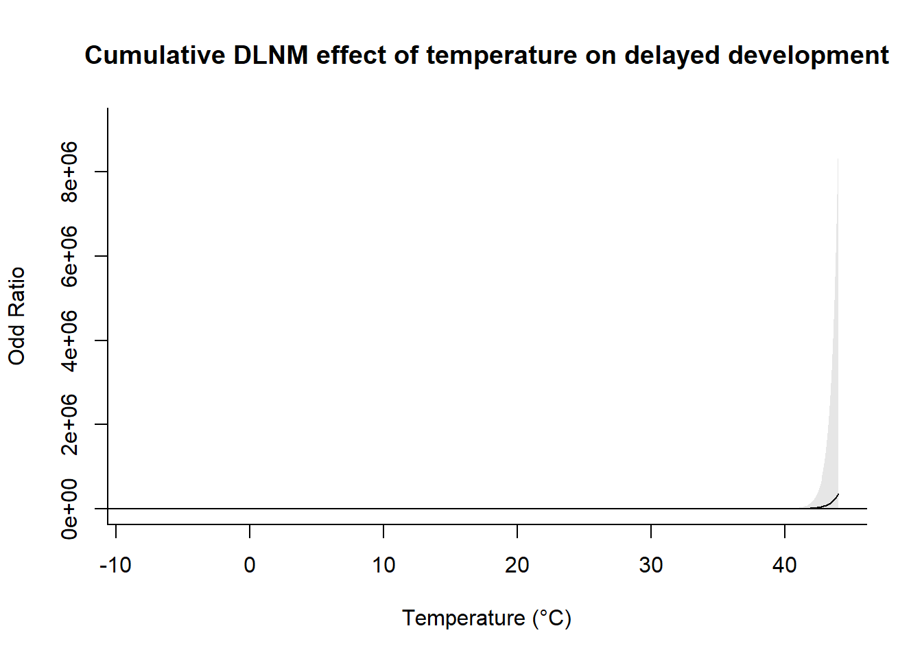
pred <- crosspred(cb_temp, model, by = 0.1, cumul = TRUE)centering value unspecified. Automatically set to 20# Plot the overall cumulative effect (adjust parameters as needed)
plot(
pred,
exp = TRUE,
"overall",
xlab = "Temperature (°C)",
ylab = "Odd Ratio",
main = "Cumulative DLNM effect of temperature on delayed development"
)
plot( pred, exp = TRUE, xlab = “Temperature (°C)”, zlab = “Odd Ratio”, theta = 220, # rotation angle phi = 35, # elevation angle ltheta = -120, # lighting angle main = “3D Graph of Temperature-Lag-HR” )
plot( pred, exp = TRUE, “contour”, plot.title = title( xlab = “Temperature (°C)”, ylab = “Lag (months)”, main = “Contour Plot of Temperature-Lag-OR” ), key.title = title(“Odd Ratio”) )