pacman::p_load(
  rio,
  here,
  dlnm,
  splines,
  survival,
  survminer,
  coxme,
  sjPlot,
  tidyverse
)Explore the association of temperature exposure with the outcome of early childhood development accross different countries
Load package and data
Data structure description: caseid_num_un is the variable that uniquely identifies each individual. Since the data is in long format, the variable case specifies the observations at the interview date (value = 1) and the temperature observations prior to the interview since birth (value = 0). If the outcome of delayed development occurs at the time of the interview, the variable delay_occ is 1, and 0 at all other timepoints.The temperature exposure is included as monthly averages of the maximum temperature (monthly_avg_tempmax) at the timepoints temp_month.
The objective is to use the dlnm analysis to explore the association of temperature exposure with the outcome of early childhood development comparing different included countries (specified in the variable dhscc).
Keep only relevant variable for dlnm analysis
Here is just an example, you can use select() function to choose more variables that you want to include in your final model.
data_dlnm <- data %>%
  group_by(caseid_num_un) %>%
  mutate(time_since_birth = temp_month - min(temp_month) + 1) %>%
  ungroup() %>%
  select(
    caseid_num_un,
    case,
    dhscc,
    delay_occ,
    temp_month_converted,
    time_since_birth,
    contains("temp")
)names(data_dlnm) [1] "caseid_num_un" "case" "dhscc"
[4] "delay_occ" "temp_month_converted" "time_since_birth"
[7] "temp_month" "monthly_avg_tempmax" "temp_lag1"
[10] "temp_lag2" "temp_lag3" "temp_lag4"
[13] "temp_lag5" "temp_lag6" "temp_lag7"
[16] "temp_lag8" "temp_lag9" "temp_lag10"
[19] "temp_lag11" "temp_lag12" "temp_lag13"
[22] "temp_lag14" "temp_lag15" "temp_lag16"
[25] "temp_lag17" "temp_lag18" "temp_lag19"
[28] "temp_lag20" "temp_lag21" "temp_lag22"
[31] "temp_lag23" "temp_lag24" "temp_lag25"
[34] "temp_lag26" "temp_lag27" "temp_lag28"
[37] "temp_lag29" "temp_lag30" "temp_lag31"
[40] "temp_lag32" "temp_lag33" "temp_lag34"
[43] "temp_lag35" "temp_lag36" "temp_lag37"
[46] "temp_lag38" "temp_lag39" "temp_lag40"
[49] "temp_lag41" "temp_lag42" "temp_lag43"
[52] "temp_lag44" "temp_lag45" "temp_lag46"
[55] "temp_lag47" "temp_lag48" "temp_lag49"
[58] "temp_lag50" "temp_lag51" "temp_lag52"
[61] "temp_lag53" "temp_lag54" "temp_lag55"
[64] "temp_lag56" "temp_lag57" "temp_lag58"
[67] "temp_lag59" "temp_lag60" "temp_spline1"
[70] "temp_spline2" "temp_spline3" "temp_spline4" The data contains the main exposure monthly_avg_tempmax, plus pre-computed lags (temp_lag1 to temp_lag60). Often in DLNM analyses, we should let the DLNM functions create the lag structure from the raw exposure. In this study, we can use monthly_avg_tempmax as the main exposure variable and specify a lag period (here, 60 months).
total_cases <- data_dlnm %>%
  group_by(caseid_num_un) %>%
  summarise(has_case = any(delay_occ == 1)) %>% # check if delayed development observed for each child
  summarise(total_cases = sum(has_case)) # count the number of child with delayed development observered
total_cases_pct <- round(total_cases * 100 / 20813, 2)
There are 8797 children observed delayed development, accounted for 42.27%
km_data <- data_dlnm %>%
  group_by(caseid_num_un) %>%
  summarise(
    time_event_since_birth = max(time_since_birth), # or time of first delay/censoring
    delay_occ = max(delay_occ), # should be 1 if delay occurred
    dhscc = first(dhscc) # keep country info
  )

km_fit <- survfit(
  Surv(time_event_since_birth, delay_occ) ~ dhscc,
  data = km_data
)ggsurvplot(
km_fit,
data = km_data,
pval = TRUE, # show p-value for log-rank test
conf.int = TRUE, # confidence intervals
risk.table = TRUE, # show number at risk below plot
legend.title = "Country",
xlab = "Months since birth",
ylab = "Survival probability (no delay)",
palette = "Set1" # or use any ggplot2 color palette
)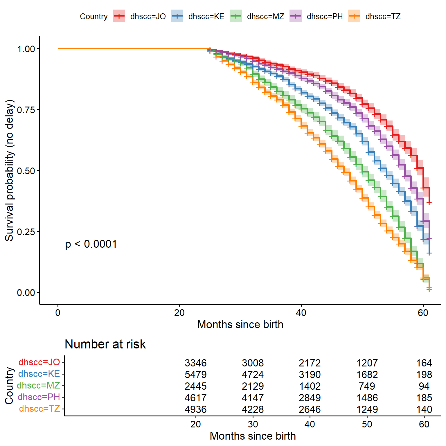
Interpretation: Lower curve = higher risk / earlier onset of developmental delay.
Recommended Analysis: Time-to-event (survival) model with DLNM
| Aspect | Description |
|---|---|
| Time scale |
temp_month provides a natural time axis (e.g., months since birth). |
| Censoring | Children who didn’t have delay by interview are right-censored at their last observation (delay_occ = 0 until end). |
| Event indicator |
delay_occ = 1 marks the first event (delay). |
| Exposure over time |
monthly_avg_tempmax is a time-varying exposure, used for DLNM to assess lagged non-linear effects. |
| Multiple countries | Use dhscc as a stratifying variable or interaction term to assess cross-country differences in effects. |
Setting Up the DLNM
lag <- 6
temp_matrix <- data_dlnm %>%
  group_by(caseid_num_un) %>%
  mutate(max_time = max(time_since_birth)) %>%
  filter(time_since_birth >= max_time - lag) %>% # lag = 6 months
  mutate(lag = max_time - time_since_birth) %>%
  ungroup() %>%
  select(caseid_num_un, lag, monthly_avg_tempmax) %>%
  pivot_wider(
    names_from = lag,
    values_from = monthly_avg_tempmax,
    names_prefix = "lag"
  ) %>%
  select(all_of(paste0("lag", 0:lag))) %>%
  as.matrix()

cb_temp <- crossbasis(
  temp_matrix,
  lag = lag, # max lag in months (example)
  argvar = list(fun = "ns", df = 4), # exposure-response basis
  arglag = list(fun = "ns", df = 3) # lag-response basis
)
model_cox_normal <- coxph(
Surv(time_event_since_birth, delay_occ) ~ cb_temp + strata(dhscc), # can add more other_covariates here
data = km_data
)
model_cox_re <- coxme(
Surv(time_event_since_birth, delay_occ) ~ cb_temp + (1 | dhscc), # can add more other_covariates here
data = km_data
)
sjPlot::tab_model(model_cox_normal, model_cox_re)| Surv(time event since birth,delay occ) |
Surv(time event since birth,delay occ) |
|||||
|---|---|---|---|---|---|---|
| Predictors | Estimates | CI | p | Estimates | CI | p |
| cb tempv1 l1 | 0.14 | 0.02 – 0.91 | 0.039 | 2.22 | 1.05 – 4.69 | 0.037 |
| cb tempv1 l2 | 0.05 | 0.01 – 0.39 | 0.005 | 1.26 | 0.64 – 2.47 | 0.509 |
| cb tempv1 l3 | 0.57 | 0.34 – 0.96 | 0.034 | 1.06 | 0.75 – 1.50 | 0.741 |
| cb tempv2 l1 | 0.27 | 0.09 – 0.83 | 0.022 | 1.48 | 1.01 – 2.18 | 0.046 |
| cb tempv2 l2 | 0.16 | 0.03 – 0.76 | 0.021 | 1.59 | 0.88 – 2.88 | 0.124 |
| cb tempv2 l3 | 0.90 | 0.66 – 1.23 | 0.504 | 1.15 | 0.88 – 1.52 | 0.305 |
| cb tempv3 l1 | 0.16 | 0.00 – 6.91 | 0.339 | 19.08 | 2.29 – 159.26 | 0.006 |
| cb tempv3 l2 | 0.04 | 0.00 – 1.42 | 0.077 | 7.34 | 1.72 – 31.33 | 0.007 |
| cb tempv3 l3 | 0.15 | 0.05 – 0.48 | 0.001 | 0.57 | 0.25 – 1.27 | 0.169 |
| cb tempv4 l1 | 1.74 | 0.60 – 5.07 | 0.308 | 1.89 | 0.68 – 5.25 | 0.224 |
| cb tempv4 l2 | 2.99 | 0.66 – 13.55 | 0.155 | 0.53 | 0.19 – 1.45 | 0.215 |
| cb tempv4 l3 | 0.90 | 0.28 – 2.92 | 0.855 | 0.39 | 0.14 – 1.06 | 0.066 |
| N | 5 dhscc | |||||
| Observations | 20823 | 20823 | ||||
| R2 Nagelkerke | 0.003 | NA | ||||
When we strata(dhscc), it means we assume the baseline hazard might be different among countries (due to healthcare systems, socialeconomic factors, etc.). The variable dhscc will not be estimated, instead data will be subseted and the coefficients are estimated. This approach assume the effect of temperature are constant across country
Random Effects: (1 | dhscc) specifies a random intercept for each country. This means the baseline hazard is allowed to vary by country, capturing unobserved heterogeneity. It helps to explain how different baseline harzard the countries are at baseline.
# Create predictions from the crossbasis
pred <- crosspred(
cb_temp,
model_cox_re,
at = c(
quantile(data_dlnm$monthly_avg_tempmax, probs = seq(0.05, 0.95, by = 0.1)),
25
),
cumul = TRUE
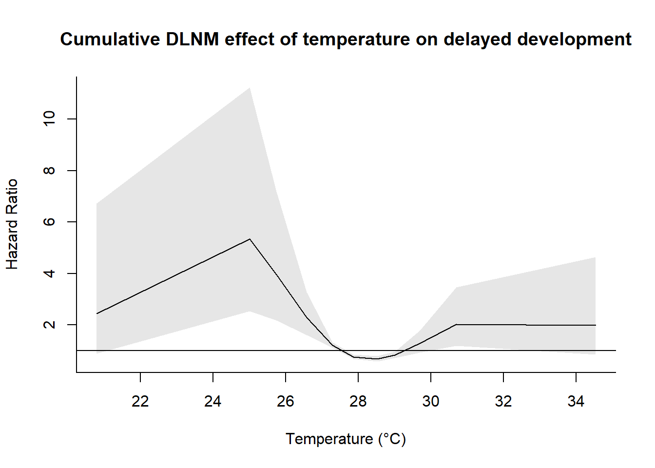
)centering value unspecified. Automatically set to 27.5# Plot the overall cumulative effect (adjust parameters as needed)
plot(
pred,
exp = TRUE,
"overall",
xlab = "Temperature (°C)",
ylab = "Hazard Ratio",
main = "Cumulative DLNM effect of temperature on delayed development"
)
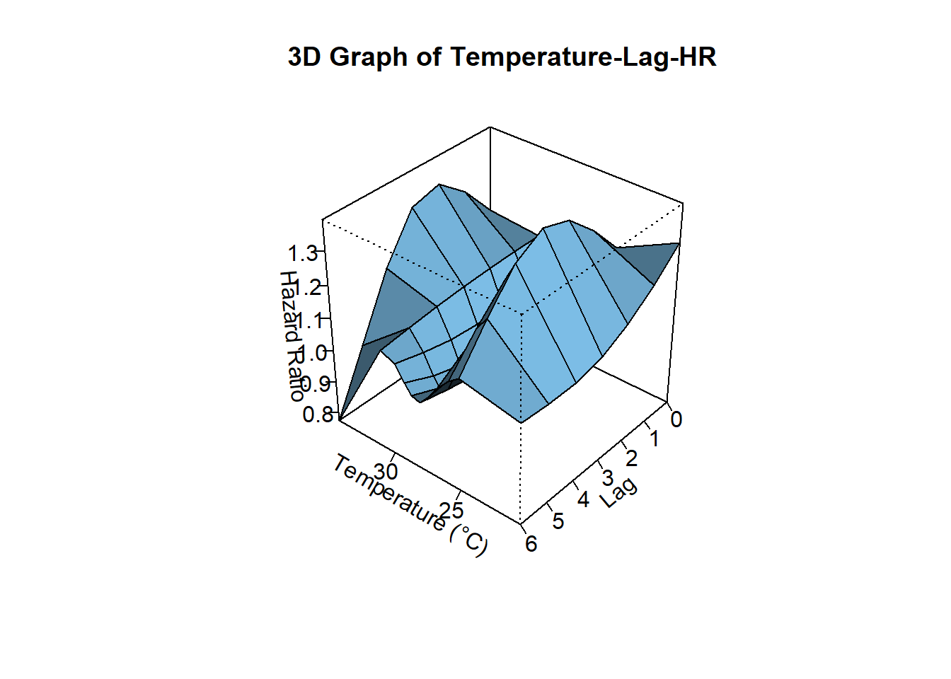
plot(
  pred,
  exp = TRUE,
  xlab = "Temperature (°C)",
  zlab = "Hazard Ratio",
  theta = 220, # rotation angle
  phi = 35, # elevation angle
  ltheta = -120, # lighting angle
  main = "3D Graph of Temperature-Lag-HR"
)